Jekyll2024-03-15T16:12:58+00:00/feed.xmlThe Twenty PercentPersonal Blog about electrical engineering, IT and finishing projects.Cyrill KünziBuilding a cute CO2 gauge2024-03-15T07:17:21+00:002024-03-15T07:17:21+00:00/co2A good smart home is one where I don’t have to fiddle around with my phone all the time.
This philosophy has manifested as several physical switches spread across the apartment, controlling most essential functions.
But especially in the winter when all windows stay shut, I found myself monitoring the room’s CO2 levels quite frequently.
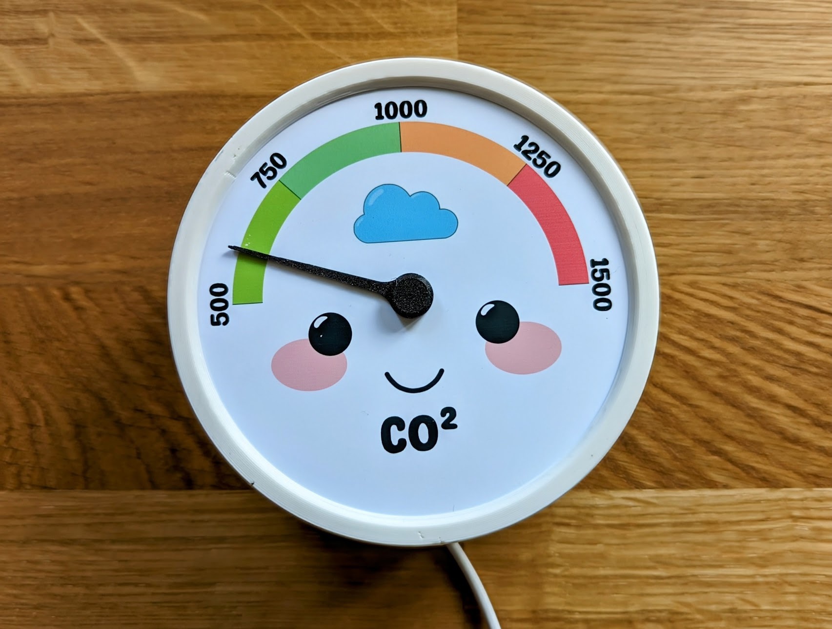
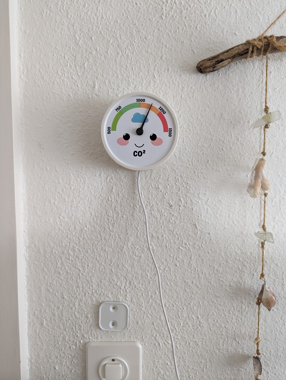
The quest to free myself from this unnecessary phone checking resulted in the following specimen:
The Hardware
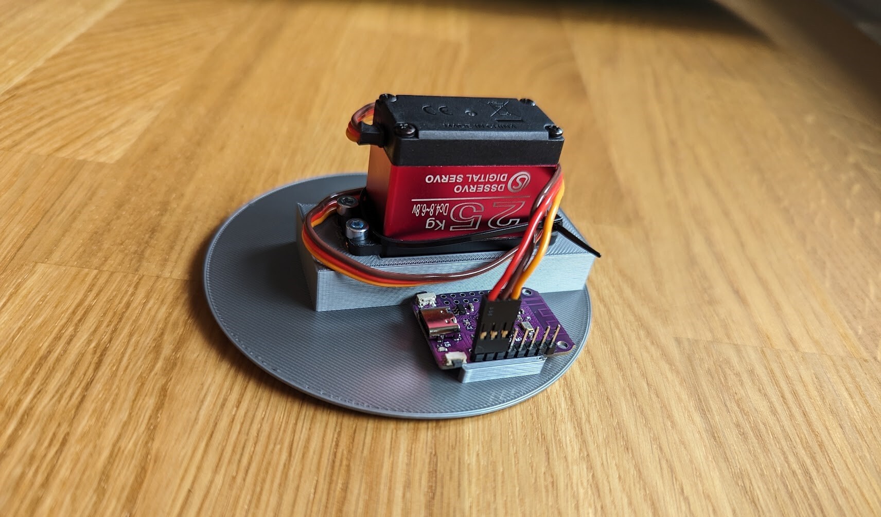
The core of the setup consists of a DS3225 servo powered by a Wemos S2 mini.
Both components were chosen by the very scientific process of already being in my drawer.
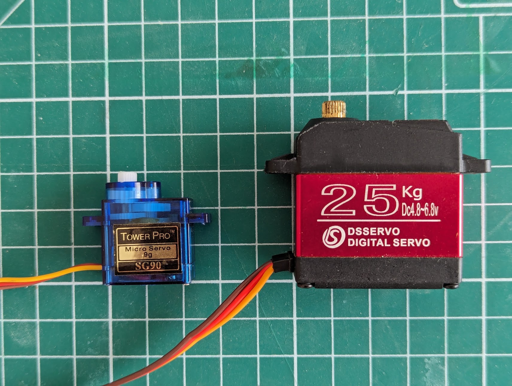
The 25 kg servo is admittedly a bit oversized for turning a tiny plastic pointer. But it is also much quieter than one of these ultra-cheap AliExpress alternatives, which is a plus when hanging in the living room.
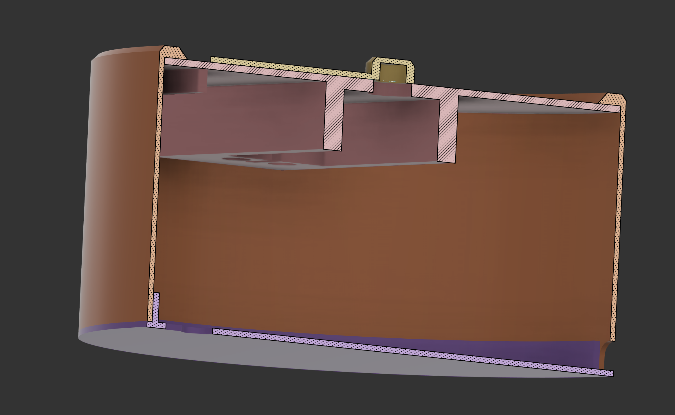
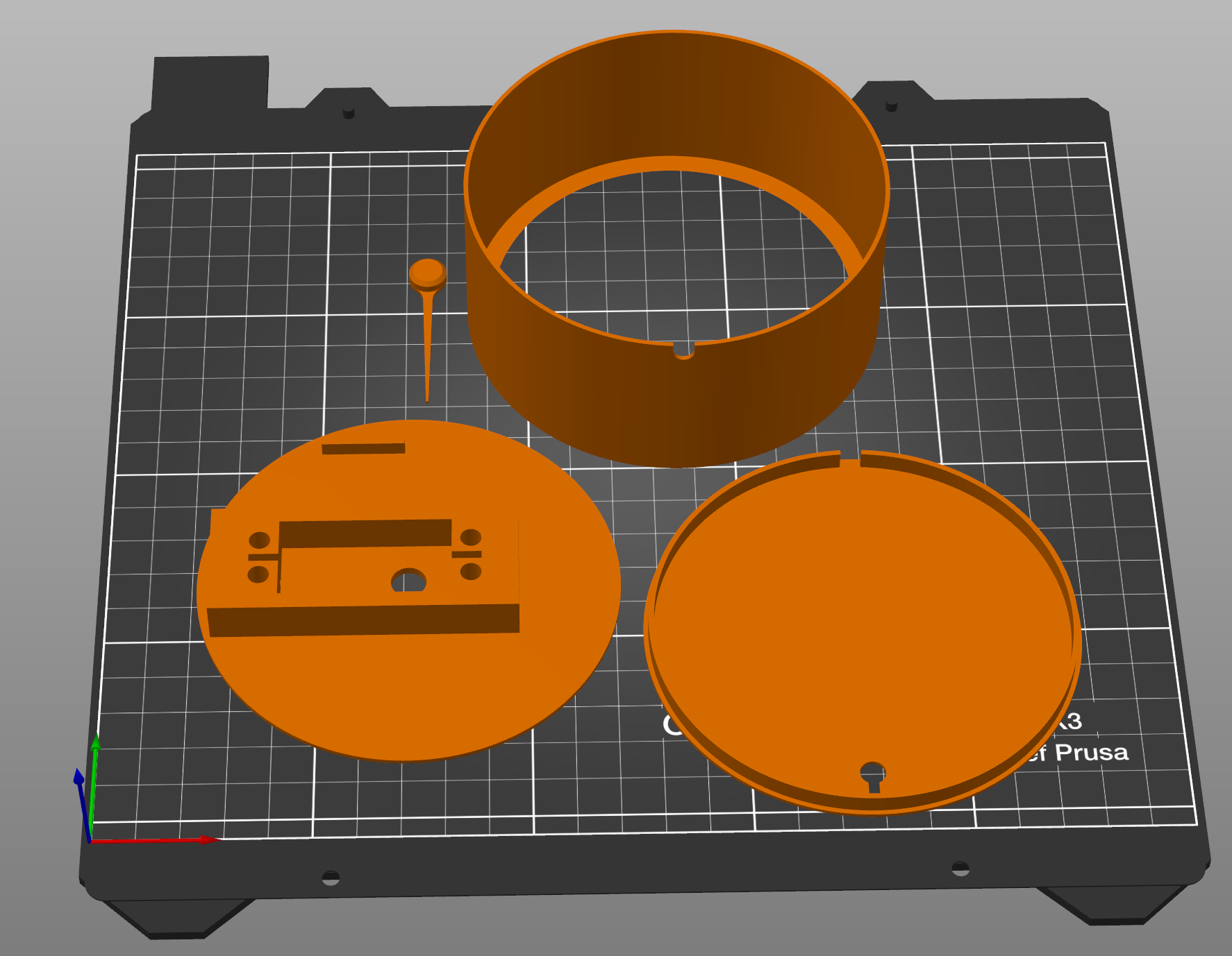
Everything is held together with either press-fits or threaded inserts, while a print-out of the gouge is sandwiched between the ‘face’ and outer casing. Crafting the artistic design was probably the toughest challenge of this project, especially for a total Inkscape noob like myself.
3D printed parts
To be able to directly plug the servo into the board, I had to swap the servo’s power and ground connections inside the dupont connector. So if you choose to recreate this design, make sure to double-check your connections to avoid any accidents.
The Software
Setup
Using ESPHome made it super easy to integrate this piece of hardware into my Home Assistant instance.
But unfortunately, their convenient web programmer doesn’t yet support the ESP32-S2 I’m using. After some digging, I found the following workaround to get everything up and running:
At this point, the board can be wirelessly updated like any other ESPHome device. There are probably other ways of doing this, like flashing directly with esptool, but this was the most convenient for me.
Board config
As you might have guessed, this device doesn’t come with its own CO2 sensor onboard. Instead, the values are relayed from another ESP32-based sensor through Home Assistant. But it would, of course, also be possible to integrate such a sensor into the same device. Just make sure to include some extra holes in the case.
The servo is configured like this:
servo:-id:pointeroutput:pwm_outputtransition_length:10s# make pointer nove slowly to reduce noiseauto_detach_time:3smin_level:2.8%# calibrate to move in a 180° arcmax_level:12.7%# calibrate to move in a 180° arcoutput:-platform:ledcid:pwm_outputpin:GPIO16# conveniently located next to 5V/GNDfrequency:50Hznumber:-platform:templatename:Servo Controlmin_value:0initial_value:50max_value:100step:0.1optimistic:trueset_action:then:-servo.write:id:pointerlevel:!lambda'return(x*2-100)/-100.0;'# map value to servo position
You might have to tinker with the min_level, max_level, or value mapping in order to get the pointer to line up perfectly with the printout.
Home Assistant config
All Home Assistant has to do is monitor changes in CO2 concentration and map/transmit the updated values to the gauge. The corresponding automation could look like this:
At this point, everything should be up and running smoothly, with the pointer responding promptly to new readings from the CO2 sensor.
Conclusion
This was a fun little project, and I like looking at the little guy nudging me to open the windows more often.
The design can also easily be tweaked to display any kind of sensor value.
If you are interested in building your own, you can find the relevant files on my GitHub.
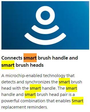
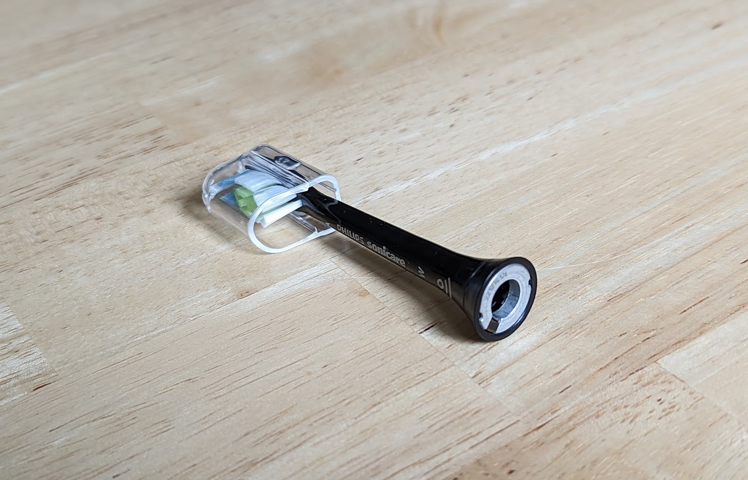
]]>Cyrill KünziHacking my “smart” toothbrush2023-05-24T09:17:21+00:002023-05-24T09:17:21+00:00/toothbrushAfter buying a new Philips Sonicare toothbrush I was surprised to see that it reacts to the insertion of a brush head by blinking an LED.
A quick online search reveals that the head communicates with the toothbrush handle to remind you when it’s time to buy a new one.
From the Philips product page: seems to be REALLY smart!
Reverse Engineering
Looking at the base of the head shows that it contains an antenna and a tiny black box that is presumably an IC.
The next hint can be found in the manual where it says that: “Radio Equipment in this product operates at 13.56 MHz”, which would indicate that it is an NFC tag.
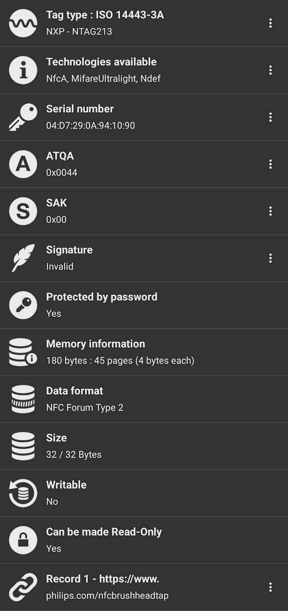
And indeed when holding the brush head to my phone it opens a link to a product page: https://www.usa.philips.com/c-m-pe/toothbrush-heads.
Using the NFC Tools app we can learn a lot about this tag:
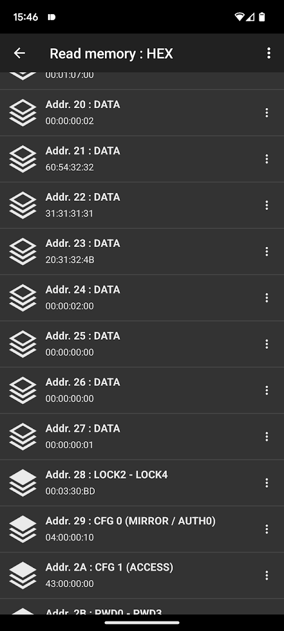
Also using NFC Tools, the memory and memory access conditions can be read:
Address
Data
Type
Access
0x00
04:EC:FC:9C
UID0-UID2/BCC0
Read-Only
0x01
A2:94:10:90
UID3-UDI6
Read-Only
0x02
B6:48:FF:FF
BCC1/INT./LOCK0-LOCK1
Read-Only
0x03
E1:10:12:00
OTP0-OTP3
Read-Only
0x04
03:20:D1:01
DATA
Read-Only
0x05
1C:55:02:70
DATA
Read-Only
0x06
68:69:6C:69
DATA
Read-Only
0x07
70:73:2E:63
DATA
Read-Only
0x08
6F:6D:2F:6E
DATA
Read-Only
0x09
66:63:62:72
DATA
Read-Only
0x0A
75:73:68:68
DATA
Read-Only
0x0B
65:61:64:74
DATA
Read-Only
0x0C
61:70:FE:00
DATA
Read-Only
0x0D…
00:00:00:00
DATA
Read-Only
0x1F
00:01:07:00
DATA
Readable, write protected by PW
0x20
00:00:00:02
DATA
Read-Only
0x21
60:54:32:32
DATA
Read-Only
0x22
31:32:31:34
DATA
Read-Only
0x23
20:31:32:4B
DATA
Read-Only
0x24
B3:02:02:00
DATA
Readable,write protected by PW
0x25
00:00:00:00
DATA
Readable,write protected by PW
0x26
00:00:00:00
DATA
Readable,write protected by PW
0x27
00:00:00:01
DATA
Readable,write protected by PW
0x28
00:03:30:BD
LOCK2 - LOCK4
Readable,write protected by PW
0x29
04:00:00:10
CFG 0
Read-Only
0x2A
43:00:00:00
CFG 1
Read-Only
0x2B
00:00:00:00
PWD0-PWD3
Write-Only
0x2C
00:00:00:00
PACK0-PACK1
Write-Only
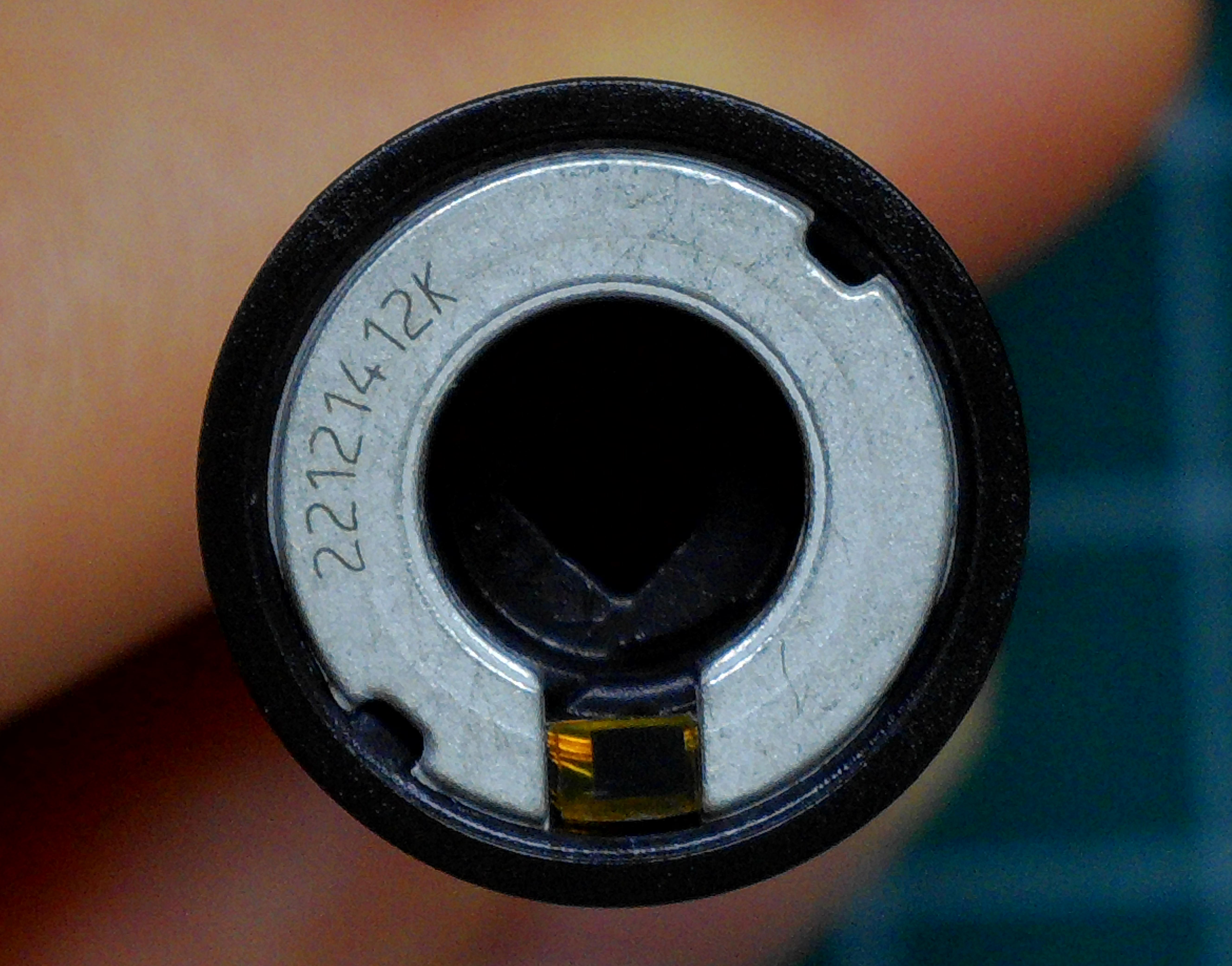
I repeated this process for one black and two white W DiamondClean brush heads and learned the following:
Address 0x00-0x02 contains a unique ID and its checksum
Address 0x04-0x0C contains the link to the Philips store
Address 0x22 is 31:32:31:34 for black and 31:31:31:31 for white heads respectively
Address 0x24 contains the total brush time
All other readable data is identical between all heads
Decoding the stored time
Let’s do an experiment to see what changes happen to the tag when using the toothbrush:
Read the tag
When reading a new brush head that has never been in contact with the data at addr. 0x24 is 00:00:02:00.
Simply attaching it to the handle (without brushing) changes nothing
Brush for some time
In this case, I let the toothbrush run for 5s
Read the tag again
The data at addr. 0x24 is now 05:00:02:00
Observe the difference
Looks like addr. 0x24 saves the number of seconds that the brush head was in use
When the brush is used for more than 255s, this timer rolls over to the second bit (02:01:02:00 -> 258s).
Trying to overwrite the stored time is unfortunately unsuccessful, as this memory address is password protected.
Sniffing the password
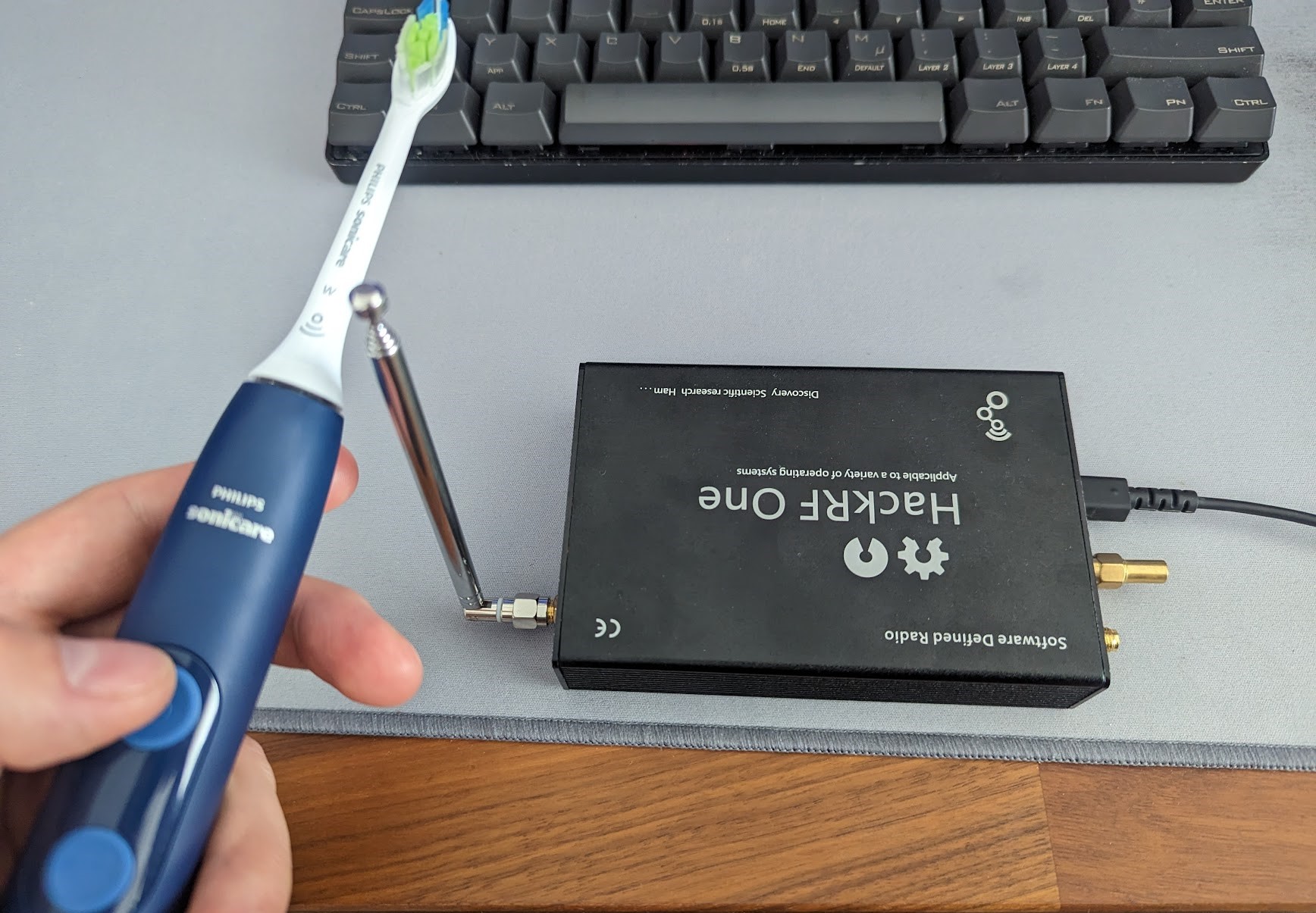
Luckily it turns out that the required password is sent over plain text! So all I need to do is to sniff the communication between the toothbrush and the head.
After digging out my HackRFsoftware defined radio and some trial and error, I came up with the following workflow.
Record RF signal
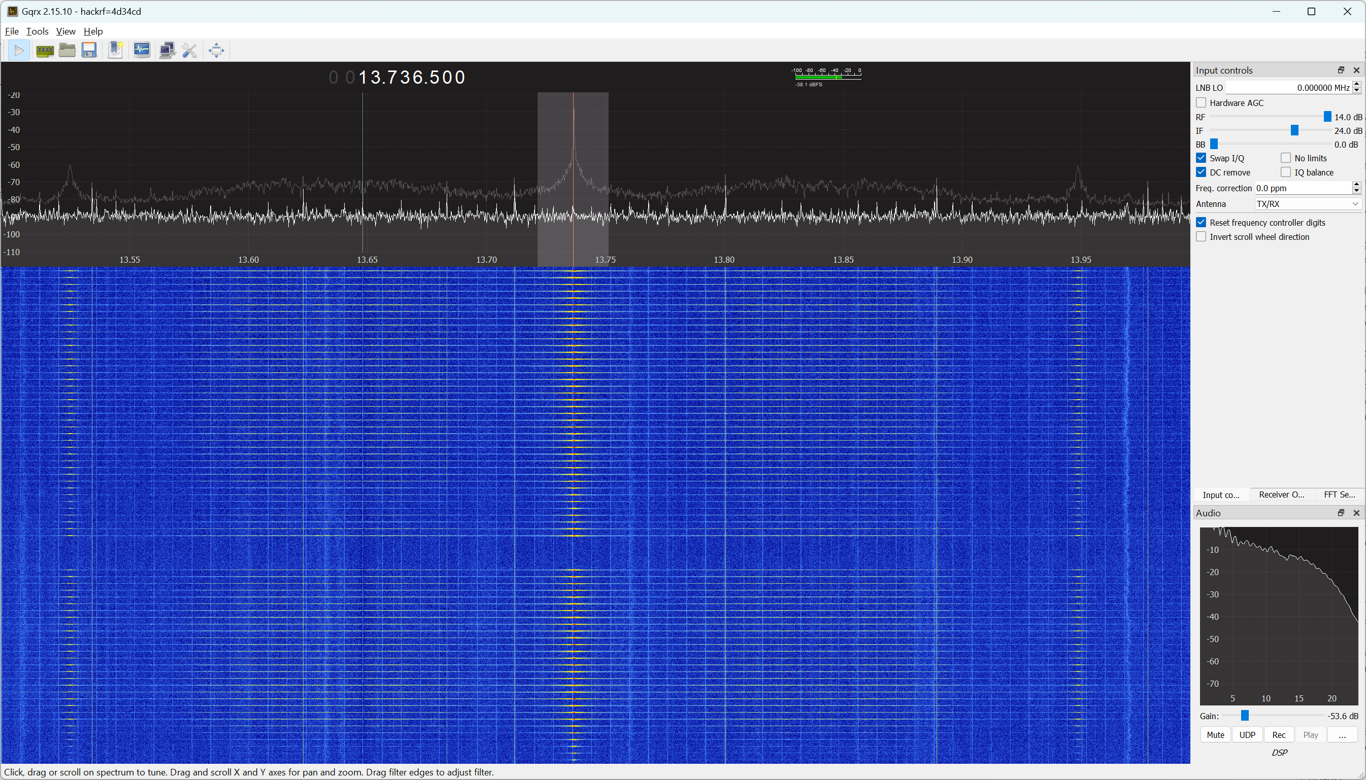
When opening gqrx and tuning it to 13.736 MHz while holding the toothbrush close to the antenna, it is visible that the head gets polled multiple times a second. It is a welcome surprise that my simple monopole antenna gets a signal that is strong enough for this purpose. You can download the relevant gqrx configuration file here.
While brushing, the NFC polling takes a brief pause and the first burst of packets that follows updates the time counter.
With the ability of gqrx to make I/Q recordings, we can capture the password RF signals like this:
Turn on the toothbrush
Start recording
Turn off the toothbrush
Stop the recording
The first packets in the file should now contain the password in plain text.
Convert recording
Before this raw I/Q file can be decoded it needs to be converted into a slightly different format to be read by the decoding program.
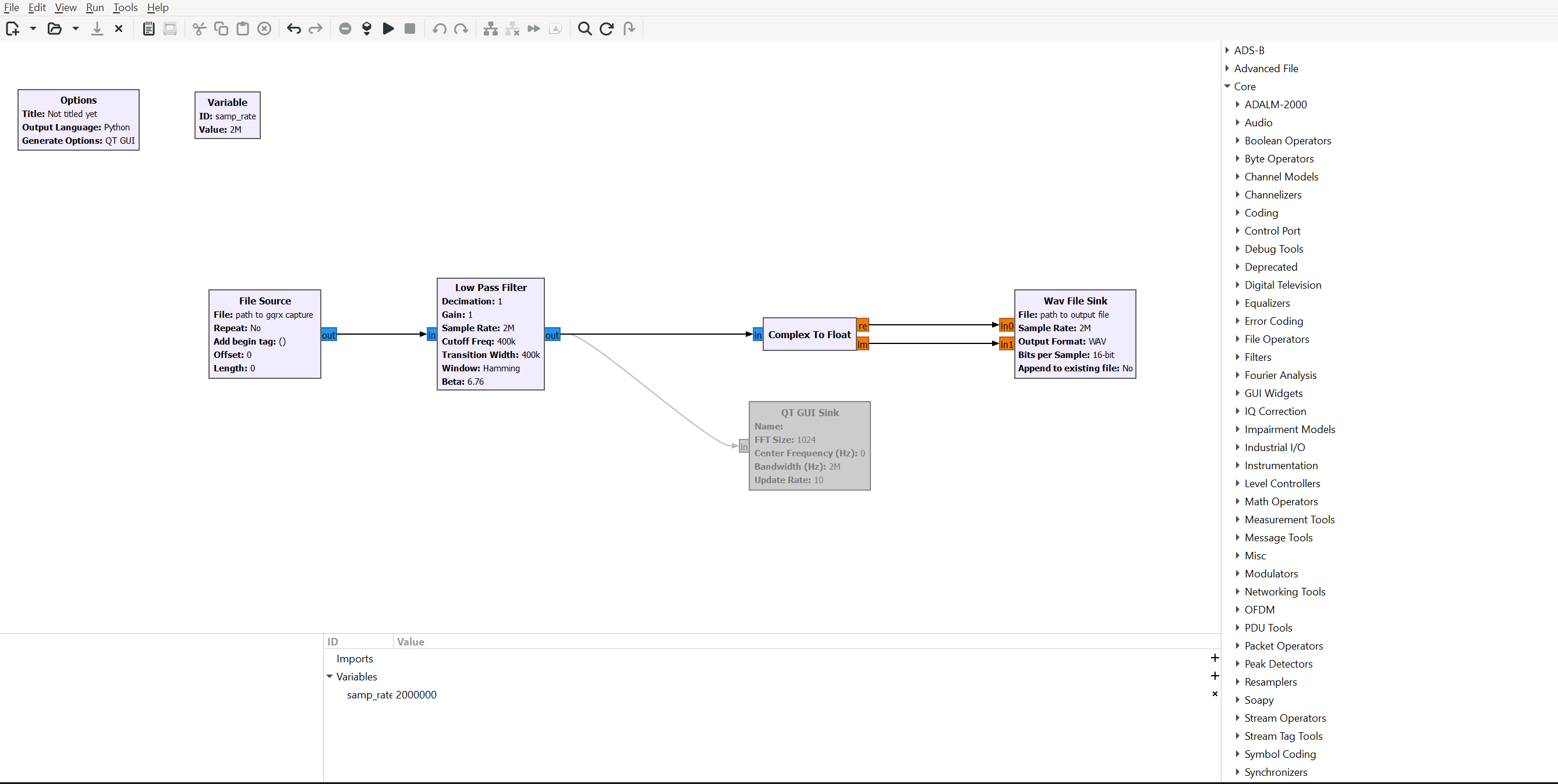
I created a small gnuradio companion script that applies a lowpass filter and converts the data into a wav file with two channels that contain the real and imaginary components of the complex signal.
Make sure to substitute the correct paths in the source/sink blocks and check the sampling frequency (I used 2MHz).
You can download the script here.
Decode recording
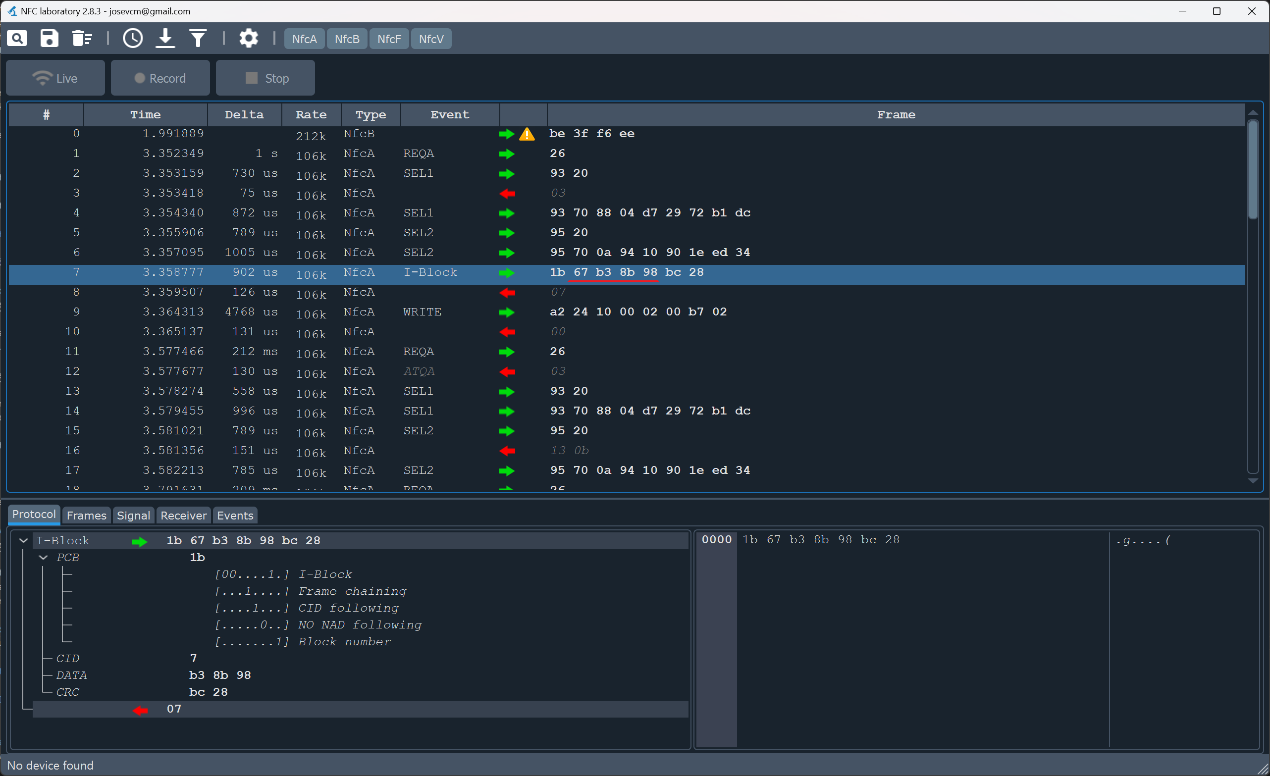
I found the perfect tool for this task called NFC-laboratory.
After opening the newly created WAV file, it should look something like the picture above. In this case, the recording is only good enough to see the communication that goes from host to tag (green arrow). But to sniff the password this is perfect.
When looking at the datasheet for the NTAG213, we can see what is happening:
Line #0-#6: communication is established with the tags’ unique ID
Line #7: The toothbrush sends the password (command 0x1B = PWD_AUTH)
Line #9: The time counter is updated to the new value (command 0xA2 = WRITE)
All lines below are repeated polling without password authentication or writing anything
So the password for this brush head is 67:B3:8B:98 (underlined in the picture).
Writing to the brush
With the password successfully acquired, it’s now possible to set the counter on the brush head to anything we want by sending the relevant bytes over NFC.
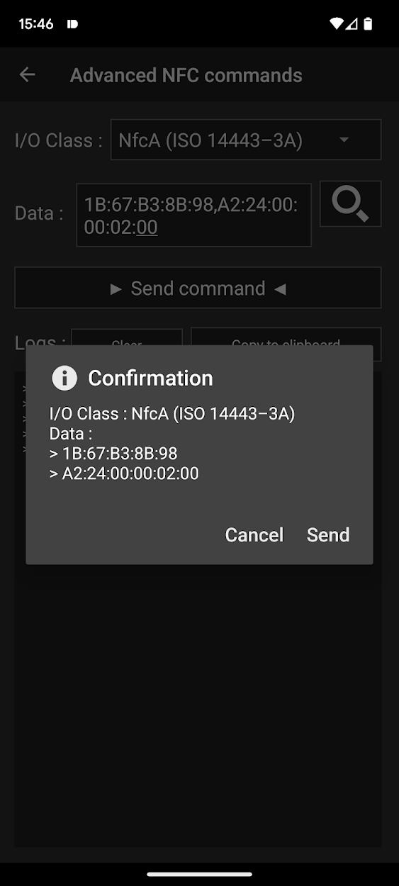
NFC Tools comes to the rescue again:
Go to Other -> Advanced NFC commands
Set the I/O Class to NfcA
Set the data to 1B:67:B3:8B:98,A2:24:00:00:02:00
Enjoy a factory-new brush head (at least as far as the time counter is concerned)
Here is the breakdown of the command in step 3:
Command
Explanation
1B
PWD_AUTH
67:B3:8B:98
The password
,
Package delimiter
A2
WRITE
24
To address 0x24
00:00:02:00
Timer set to 0s
Below you can see the memory of the brush head before and after the custom NFC commands:
Observe how the timer at address 0x24 changes
With this, the toothbrush is now successfully hacked and we can play around with the timer as we wish.
Here are some interesting observations:
Only the first two bytes at address 0x24 are used for timekeeping. Once the counter reaches FF:FF:02:00 it stops going up (18 hours of continuous brushing).
When the stored time is greater than 0x5460 the toothbrush blinks the LED to notify you to change heads. This corresponds to 21’600s -> 180 x 2min -> 3 months of brushing twice a day, which is exactly in line with Philips recommendation to change heads every 3 months.
Final Remarks
Password verification protection
You might have noticed the color of the brush head changing throughout of this post. This is because I had to run out and buy a new one after getting locked out of the first one.
When having a close look at the contents of address 0x2A which is 43:00:00:00 and page 18 of the datasheet, we can see that the tag is configured to permanently disable all write access after three wrong password attempts. (Which I promptly exceeded when playing around) This means that not even the toothbrush handle itself can write to this head again.
Password generation
Unfortunately, the password of every brush head is unique and this process of extracting it with an SDR is quite involved and requires special hardware.
At the bottom of page 30 in the datasheet, NXP recommends generating the password from the 7-byte UID. Below are all the UID - password pairs I obtained from my 3 heads:
UID
Password
04:79:CF:7A:89:10:90
FF:34:CE:4C
04:EC:FC:A2:94:10:90
61:F0:A5:0F
04:D7:29:0A:94:10:90
67:B3:8B:98
All my tries to guess to one-way function for generating the passwords failed. Depending on the care that the Philips engineers took, guessing this function could be almost impossible.
But if you manage to solve this puzzle, feel free to hit me up with an E-mail.
Update (August 16, 2023)
After publishing this article, I was pleasantly surprised to see it picked up by some big news sites such as Hacker News and Hackaday. The resulting discussions and comments proved to be both enlightening and entertaining. Thanks to everyone who dropped positive comments and messages!
A special shoutout has to go to Aaron Christophel who got inspired by this post to:
Dump and reverse engineer the Philips Sonicare firmware to extract the password generation algorithm: Video
And just for fun, he made the toothbrush bust out a Rick Roll
Please go check his content if you are interested in the solution to the puzzle.
]]>Cyrill KünziLanguage modeling journey: From bigram prediction and DIY transformers to LLaMA 65B2023-03-15T14:17:21+00:002023-03-15T14:17:21+00:00/llm
With all the hype surrounding chatGPT (and now GPT-4), it really bothered me that I don’t have the faintest idea of how language models or transformers work.
Fortunately, the Neural Networks: Zero to Hero lecture series that helped me understand backpropagation in my previous post, also covers multiple language modeling techniques.
I found that I spend too much time in my last post explaining things that were already covered much better in the lecture. So I’ll try to keep this one shorter.
Goal
The project has the very open-ended goal of “Learning about language models”. I don’t have millions to spend on GPU time to train the next chatGPT, so I’m going to be happy with understanding the underlying theory and training some toy models.
These are the rough goals I want to achieve:
In this post, I’m going to follow lectures 2 through 7 pretty closely. They start with creating a very simple bigram prediction model and then introduce incrementally more complex models.
Bigram model (729 parameters)
The first step is creating a character-level bigram model: It takes a training text and counts how many times a character follows another. These counts are then normalized and converted to probability distributions.
After converting the ASCII characters to integers, all bigrams are counted and the results are stored in a 2D array. In this case, each word is a name and the model will try to predict a new name.
bigram_counts=torch.zeros(27,27,dtype=torch.int32)forwordinwords:word='.'+word+'.'forc1,c2inzip(word,word[1:]):bigram_counts[stoi[c1],stoi[c2]]+=1# Get probability distribution
P_bigram=bigram_counts/bigram_counts.sum(1,keepdims=True)
Something interesting to note is that the words are surrounded by a special character ‘.’ to indicate the start and stop of each sequence. This is useful because generation can be started with a ‘.’ and the model itself can then decide when to stop by generating another ‘.’
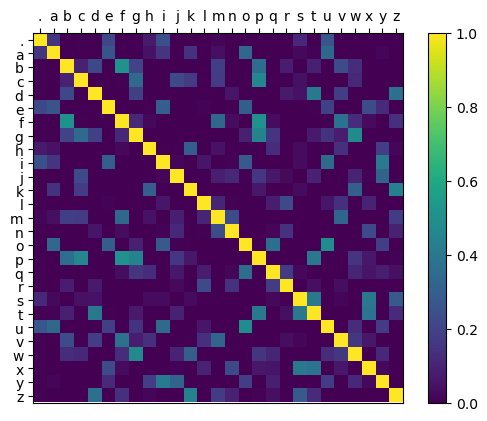
After feeding roughly 30’000 names into the model it produces the following probability distribution:
Figure 1: Bigram probability distribution generated by simple counting
As we can see, the model has learned that a lot of names start with ‘a’ and that ‘q’ is almost always followed by ‘u’.
As expected, when we use these probabilities to generate random new names, the results aren’t very good.
.myliena.
.r.
.a.
.ahi.
.grammian.
.n.
.xxonh.
.chaldeiniy.
.bler.
.jaranige.
Because the model only sees the previous character in the sequence, it doesn’t know the length of the generated name. So ‘.a.’ is a perfectly fine choice, as ‘a’ is a common letter at the start and the end of names (see figure 1).
Now with gradient descent (729 parameters)
Instead of explicitly calculating the matrix by counting, the probabilities can be learned with backpropagation and gradient descent.
In the following snippet X is the one-hot encoded input character and y is the next character in the sequence. W takes the place of P_bigram from the last section.
After training for a bit, W converges to the following distribution, which looks the same as the one in Figure 1:
Figure 2: Bigram probability distribution generated by backpropagation
This is confirmed when generating random names with the same seed, as the results are exactly the same.
.myliena.
.r.
.a.
.ahi.
.grammian.
.n.
.xxonh.
.chaldeiniy.
.bler.
.jaranige.
Multi-layer perceptron (8’762 parameters)
One straightforward way to improve the model is to increase its context length. In this case, instead of only seeing the previous character, the model is going to see the previous 3 characters.
If we just used the previous technique, the resulting 4-dimensional probability matrix would have \(27^4=531'441\) parameters, which is starting to get pretty big.
So the purely statistical approach is ditched in favor of a small feed-forward neural network defined like this:
This introduces the concept of an embedding which maps each 27-dimensional one-hot encoded input character to a 5-dimensional embedding that is learned together with the rest of the network.
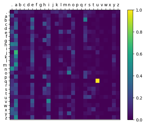
We can take a look at the cosine similarities between all embeddings after training:
Figure 3: ReLU of the cosine similarities between learned embeddings
It looks like the embeddings of the vowels are often similar to each other and that ‘.’, ‘n’, and ‘q’ have pretty distinct embeddings.
The random names generated with this model are already way better than before:
.mylieke.
.rada.
.erackanolando.
.yusamailem.
.karlymandrah.
.parlif.
.meilae.
.ayy.
.saiora.
.jaylianyyah.
WaveNet (176k parameters)
The next step is extending the context length even further and using another network topology with much more parameters.
This topology is a WaveNet introduced in 2016 by Google DeepMind https://arxiv.org/abs/1609.03499.
As seen in Figure 4, it uses dilated causal convolutions and was originally created for speech synthesis.
In this case, the convolutions are replaced with carefully arranged linear layers and the network is of course used for character prediction.
After training this network for a couple of epochs with a decreasing learning rate, the generated names start to sound pretty name-like:
.kynnale.
.obagann.
.evanne.
.jatetton.
.adiliah.
.kiyaen.
.nalar.
.khfi.
.keilei.
.awyana.
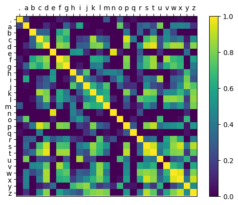
Looking at the embedding similarities again, it seems like they are more unique than before. This makes sense considering the dimensionality of the embedding vector has gone up from 5 to 20 Dimensions.
Figure 5: ReLU of the cosine similarities between learned WaveNet embeddings
GPT from scratch (10.7M parameters)
Learning how transformers work was definitely the most exciting part of this project for me!
Explaining transformers is no easy task, so I’m not even going to try. If you are interested, I highly recommend watching the lecture.
But I want to quickly show what lies in the heart of a transformer: The self-attention mechanism:
For each input, it generates a query, key, and value that get combined, such that they can exchange information with each other in a very elegant way.
The final model has 384 embeddings, a context size of 256 characters, and consists of 6 transformer blocks with 6 self-attention heads each.
After being trained on the works of Shakespeare for a couple of thousand epochs (on the GPU this time), it produces text like this:
And come to Coriolanus.
CORIOLANUS:
I will be so, show; I hope this service
As it gives me a word which to practise my lave,
When I had rather cry ‘‘twas but a bulk.
MENENIUS:
Let’s not pray you.
AUTOLYCUS:
I know ‘tis not without the shepherd, not a monster, man.
CORIOLANUS:
The poor, Pampey, sir.
CORIOLANUS:
Nor thou hast, my lord; there I know the taple
I was violently?
CORIOLANUS:
Why, that that he were recounted nose,
A heart of your lord’st traded, whose eservice we remain
With this chance to you did
The deputy of such pure complices them
Redeem with our love they call and new good to-night.
BRUTUS:
I dare now in the voices: here are
Acrown the state news.
SICINIUS:
You have been in crutching of them, cry on their this?
MENENIUS:
Proclam, sir, I shall.
Playing with LLaMA (65B parameters)
While doing this project the weights of Facebooks LLaMa model leaked online in a hilarious way.
When looking at their publicly available model, most things seem very similar to the DIY version.
Language models might start having their StableDiffusion moment right now. Seemingly every day there is a new innovation like reducing the model size with quantization or finetuning it to act more like OpenAIs Davinci model.
After increasing my WSLs RAM budget to 50GB, downloading the LLaMA weights and quantizing them to 4-bit, I was able to use llama.cpp to run the 65B model on a CPU.
Like with diffusion models, it seems futile to go into much detail here, as the whole landscape will probably look completely different in only a couple of weeks.
Conclusion
Going from having absolutely no clue about LLMs and transformers to understanding the current cutting-edge research was definitely a fun project.
Major props have to go to Andrej Karpathy for his amazing lectures that perfectly guided me through this process.
I will probably return to this topic soon when the available models and tooling have advanced enough to do DIY fine-tuning.
All code can be found on my GitHub
]]>Cyrill KünziWriting an autograd engine and creating images with backpropagation2023-02-23T15:54:21+00:002023-02-23T15:54:21+00:00/nanogradAs part of my master thesis, I implemented a spiking neural network from scratch on a microcontroller.
Because training was done separately on a PC, I only had to write the forward pass. This was a big relief because PyTorches autograd always seemed like black magic to me (even after learning the theoretical background).
So seeing a post on HackerNews about Andrej Karpathys amazing video series on building neural networks from scratch, seemed like the perfect opportunity to fix this blind spot of mine. That means this project will probably be heavily inspired by his micrograd.
Goal
The goal is to create the whole machine-learning pipeline from scratch and successfully use it to learn a task.
Implement a neural network pipeline from scratch (forward and backward pass, SGD)
Don’t use any machine learning libraries (including NumPy)
For a couple of weeks, I watched the first video in Andrej Karpathys Neural Networks: Zero to Hero
series. With the help of a Jupyter notebook, he implements a version of micrograd that implements everything from backpropagation to the ability to learn a simple binary classification task with a multilayer perceptron. In my opinion, the explanations are done exceptionally well, relying mostly on code to explain the concepts (as opposed to equations, as many university courses would).
But sometimes that feeling of understanding can be deceitful: Even when something is well understood in theory, actually using it in an exercise or a real word application can often reveal some blind spots or unforeseen difficulties.
Computational graph and backpropagation
So let’s finally start writing code! I use a Jupyter notebook for this, as it is very convenient for quick prototyping.
The first task is implementing the forward pass that builds a directed acyclic graph which remembers the order of all executed operations. Every operation takes some input vertices (each representing a number) and produces one output vertex (the result of the operation). Addition would look something like: a(child) + b(child) = c(parent)
The harder part that lies at the heart of backpropagation is the backward() function that propagates a gradient from the parent to its children. This backward function explicitly spells out the partial derivative for each operation. For example, an addition during the forward pass distributes the gradient of the parent to all children during the backward pass.
One interesting aspect of doing backpropagation on the whole graph is that it needs to be done in the correct order so that each gradient is fully computed before propagating it further. This order can be computed by using something like topological sorting. This is an item that cost me a lot of time because I had an undiscovered bug in my topo sort that would put a parent vertex in the wrong position with respect to its descendants.
Multi-layer perceptron
With the hard part out of the way, the previously defined operations (such as add and multiply) can be composed together into larger functions:
A fully connected linear layer that does matrix multiplication and adds a bias (This also stores the weights of the network)
At this point the neural network is complete and can be trained by repeating the following steps:
Feed data into the network
Predict an outcome from this data
Compare with the true outcome to calculate the loss
Backpropagate the loss throughout the network to calculate the gradients
Subtract the gradients from their weights/biases (with an appropriate learning rate)
With these steps implemented, the network can successfully learn a simple classification task such as the moons dataset
Training larger models
At this point, it seemed trivial to just do the same thing for MNIST. Unfortunately, I was confronted with the fact that this implementation of backpropagation is very very slow! Even Andrej himself said “It’s the slowest autograd engine imaginable” on Twitter. Training a model on only a handful of the 60’000 28x28 images of MNIST already took several minutes. Even after moving the goalpost to a smaller dataset with 8x8 images, training was prohibitively slow.
At this point, I decided that I learned everything I wanted to learn from this project and throw in the towel regarding the goal of learning MNIST.
Going on a tangent
During the lecture, there was an offhand comment on how the gradients are also unnecessarily computed for all input values (the training images). This made me want to see if it’s possible to generate images with backpropagation.
Training 8x8 digits with PyTorch
First I had to train a decent classifier on the digits dataset. For this, I ditched my own implementation and used PyTorch which will speed up development and computation time by several orders of magnitude.
The model is a very straightforward three-layer MLP with a bit of dropout for regularization
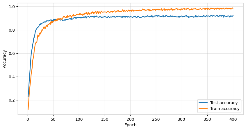
The data is split 80%/20% into a train and a test set. The training goes well, with the model achieving a final 93% accuracy on the test set.
Generating images with backprop
The goal is to generate images that look as much like a digit to the network as possible.
This is done by doing something very similar to training, but instead of the network parameters, the input image is modified with gradient descent.
In this case, the individual pixels are also clamped between 0 and 16 to match the dataset.
# seed: Array of 64 initial pixels
# target: number between 0-9
# output: Array of 64 modified pixels
defgenerate_digit(seed,target):image=seed.clone()image.requires_grad=True# This is the important part
image_optimizer=optim.Adam([image],lr=0.1)#This is like doing epochs during training
forstepinrange(100):image_optimizer.zero_grad()pred=model(torch.clamp(image,0,16))# Same loss as in training
loss=F.cross_entropy(pred,torch.tensor(target))loss.backward()image_optimizer.step()# Clamp s.t. the domain stays the same
returntorch.clamp(image,0,16)
With this, we can convert a 0 to be recognized as an 8 by the network
Generating an 8 from zero
But usually, the perception of the network does not align very well with the one of us humans! Here are the optimal digits generated from a black square:
0 1 2 3 4
5 6 7 8 9 Digits created from black squares
If you squint your eyes hard enough you might see some rough shapes for 0, 2, 3, and 5.
Another thing we can do is generate a bunch of images from noise and average them into a single composite image. In this case for each digit 1000 versions are generated from uniform noise and then averaged:
0 1 2 3 4
5 6 7 8 9 Average digits created from noise
With some more eye squinting, you might even see the 0, 2, 3, 4, 5, 7, and 8!
It is no StableDiffusion, but nonetheless a fun exercise in using backpropagation in an unusual way.
Generating adversarial images
We can also modify the loss function to simultaneously optimize toward a target digit while staying as close to the starting point as possible:
forstepinrange(100):image_optimizer.zero_grad()pred=model(torch.clamp(image,0,16))# This is the same as before
loss=F.cross_entropy(pred,torch.tensor(target))# Additional loss from difference to the original image
loss+=MSE(image,seed)*2loss.backward()image_optimizer.step()
For example, the image on the left is correctly read as an 8. But the one on the right, after being altered by the code above, is incorrectly predicted to be a 9.
Left: Origianal, read as 8 Right: Adversarial 9 with just a bit of noise
Conclusion
Unfortunately, I was not able to achieve all the initially stated goals because I didn’t achieve 80% accuracy on MNIST with my own backpropagation. I knew this was a pretty ambitious task, but did not expect it to be this hard. Maybe I was a bit spoiled by using well-optimized machine-learning libraries for years now, never appreciating how much slower they could be.
But I’m still happy with the outcome of this project, having learned a lot about backpropagation and gradient descent! Also, the tangent about generating images with backprop was quite fun, mostly because of the visual aspect and not knowing what outcomes to expect.
I think for future learning projects like this it would be a good idea to state the initial goal as something more like “Understand backprop” instead of technical milestones.
Ever since I first discovered how to print my own name with the Windows command line as a child, I’ve been drawn to all kinds of programming projects. Many years later I blinked the first LED with an Arduino and the scope of my personal projects quickly expanded to the physical realm. So over time and many projects, I’ve accumulated an impressive pile of demos, proof of concepts, and mostly finished PCBs. Unfortunately, I’ve come to the realization that the number of projects I’ve actually completed to a satisfactory degree is rather small.
Why projects fail
The cycle of starting 100 projects and finishing none is probably something that a lot of people are familiar with. There are many reasons why the initial enthusiasm oftentimes quickly fizzles out: Lack of time or motivation, unforeseen obstacles, unrealistic expectations, fear of failure, or crippling perfectionism.
I’ve fallen victim to all of these things, but generally, they happen at a point where the basic mechanism is completed, but the final touches are still missing. In these situations the 80/20 rule often comes to mind: It says that 80% of the work can be done within 20% of the time. But this also means that the final 20% (the finishing touches) take 80% of the time. This is the reason for this blog currently being called “The Twenty Percent”.
Box of mostly half-finished projects
Trying to be better
Just having completed my master’s degree puts me in a comfortable position with lots of free time and motivation to do cool things. I would like to use this opportunity to improve my ability to successfully complete personal projects. This especially means focusing on completing the elusive last 20% of the project which takes so much effort to do.
For that reason, I’m creating this personal blog to document my progress and also get some writing practice. In the beginning, the goal is to complete a few simpler projects to hone in on the process, before advancing to more complex topics later on.
The post for each project will have three sections:
Goal: Specification of the things I want to achieve with the project. When these things are done, the project is considered “complete”. But some moving of the goalpost will probably be inevitable…
Documentation: Description of the project itself, including technical details, design decisions, and challenges.
Takeaway: Analysis of the process itself, including what went well, what could be improved, and any lessons learned.
Box of 3D printed learning opportunities
First Project: Creating this Blog
Setting up this site is a perfect opportunity for a first project.
Goal
I don’t have a lot of experience with blogs or writeups, so the exact specifications of this blog will probably only be clear once I start using it. But there are some rough goals that I want to achieve:
Host the site on GitHub (or some other free alternative)
With a relatively good picture of the final product in mind, I can start working on the project.
Choosing a site generator
Going with Jekyll was the obvious choice, as it is well supported and endorsed by GitHub pages themselves and enables post creation with markdown. It also seems to have a nice trade-off between ease of use and customizability.
I chose to go with a local Jekyll install because the ability to immediately see any changes locally, significantly speeds up the process of tinkering around. Even though I don’t have any experience with Ruby, the initial setup went very smoothly and I had the example blog running in no time.
Hosting on GitHub
GitHub even has its own documentation on how to setup a Jekyll blog which surprisingly worked without a hitch. I chose to host it as my user page on ckuenzi.github.io, as it will serve as a landing page for all things concerning my projects.
Using a custom domain
Free hosting on GitHub is nice and all, but using a custom domain elevates it to the next level. Luckily this can be done rather easily by changing some DNS records. The hardest part was being patient for an hour until the DNS changes were active and the certificate was generated.
Making it look pretty
The default minima Jekyll theme already looks nice, but I decided to go with the dark version of the very popular minimal-mistakes theme because it looks a bit more modern and seems to have a lot of nifty features. The nice thing about a program like Jeykll is that the actual posts are written completely independently of the theme, which can easily be changed later.
But even with a complete theme, there are a lot of screws to turn and styles to try. This is a part of the project that I spent a lot of time on, especially because of the sophistication of this particular theme. There are still some things that I would like to improve such as including header images and a side-bar.
But no matter the theme, this site will look a bit barren without the actual content.
Writing the first post
With all the technical aspects working, this is the point where I reached my last 20% for this project. Writing this post took way longer than expected, taking a lot of perseverance and motivation. And with the hype surrounding ChatGPT at the moment, it required a lot of restraint to not outsource all the work to an LLM.
There are many things that I’m not yet sure of, such as the writing style/tone and the actual content for this blog. But these things will hopefully become more apparent with time and additional content.
Takeaway
When this subsection is written, I successfully completed my first Project. All the technical stuff was pleasantly straightforward without any unforeseen difficulties. It was also interesting to actively observe the dip in motivation once I had to start writing, which easily took 80% of my effort. It will also be interesting how that plays out with future projects that are not this meta and need writing in addition to the rest of the challenges.
For the future, it would be lovely to not procrastinate as much as I did once the hard part inevitably showed up. But carefully observing the dip in motivation and the experience of having pushed through will hopefully help with that.
In the end, I’m satisfied with the outcome of this project, as all of the goals were satisfied and I now have a product that can be easily used for future posts.


 Box of mostly half-finished projects
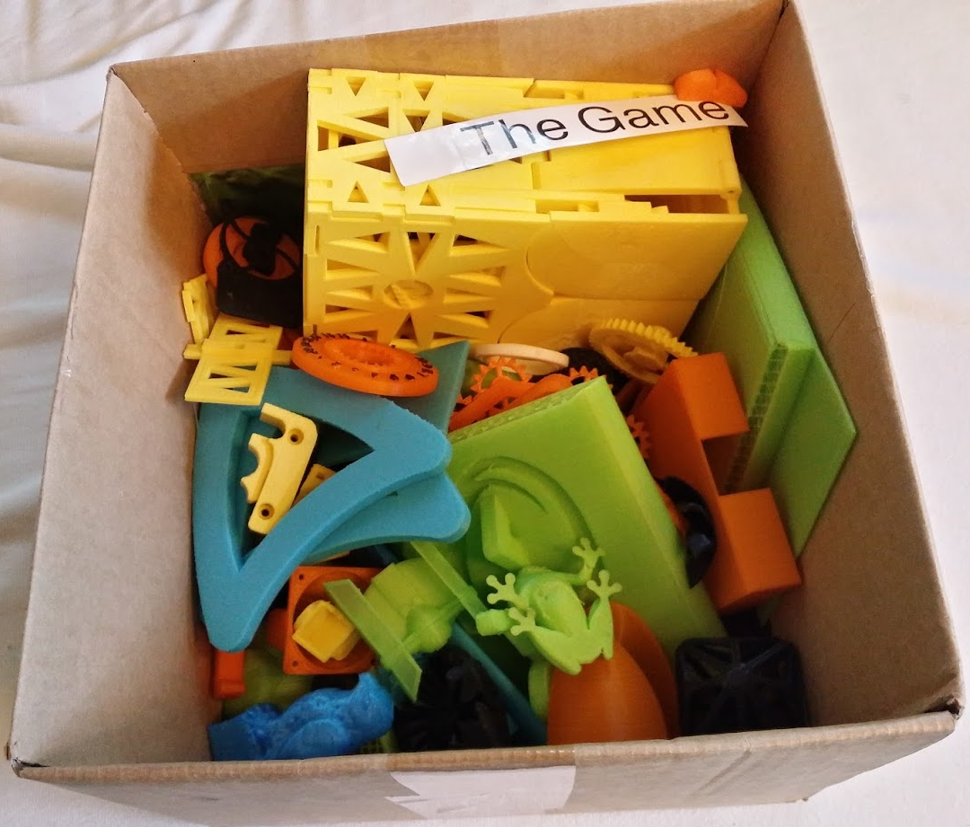 Box of 3D printed learning opportunities