Writing an autograd engine and creating images with backpropagation

7 minute read

As part of my master thesis, I implemented a spiking neural network from scratch on a microcontroller. Because training was done separately on a PC, I only had to write the forward pass. This was a big relief because PyTorches autograd always seemed like black magic to me (even after learning the theoretical background). So seeing a post on HackerNews about Andrej Karpathys amazing video series on building neural networks from scratch, seemed like the perfect opportunity to fix this blind spot of mine. That means this project will probably be heavily inspired by his micrograd.

Goal

The goal is to create the whole machine-learning pipeline from scratch and successfully use it to learn a task.

Implement a neural network pipeline from scratch (forward and backward pass, SGD)
Don’t use any machine learning libraries (including NumPy)
Get decent accuracy on MNIST, let’s say 80%

Documentation

Watching the lecture

For a couple of weeks, I watched the first video in Andrej Karpathys Neural Networks: Zero to Hero series. With the help of a Jupyter notebook, he implements a version of micrograd that implements everything from backpropagation to the ability to learn a simple binary classification task with a multilayer perceptron. In my opinion, the explanations are done exceptionally well, relying mostly on code to explain the concepts (as opposed to equations, as many university courses would).
But sometimes that feeling of understanding can be deceitful: Even when something is well understood in theory, actually using it in an exercise or a real word application can often reveal some blind spots or unforeseen difficulties.

Computational graph and backpropagation

So let’s finally start writing code! I use a Jupyter notebook for this, as it is very convenient for quick prototyping.
The first task is implementing the forward pass that builds a directed acyclic graph which remembers the order of all executed operations. Every operation takes some input vertices (each representing a number) and produces one output vertex (the result of the operation). Addition would look something like: a(child) + b(child) = c(parent) The harder part that lies at the heart of backpropagation is the backward() function that propagates a gradient from the parent to its children. This backward function explicitly spells out the partial derivative for each operation. For example, an addition during the forward pass distributes the gradient of the parent to all children during the backward pass.
One interesting aspect of doing backpropagation on the whole graph is that it needs to be done in the correct order so that each gradient is fully computed before propagating it further. This order can be computed by using something like topological sorting. This is an item that cost me a lot of time because I had an undiscovered bug in my topo sort that would put a parent vertex in the wrong position with respect to its descendants.

Multi-layer perceptron

With the hard part out of the way, the previously defined operations (such as add and multiply) can be composed together into larger functions:

A fully connected linear layer that does matrix multiplication and adds a bias (This also stores the weights of the network)
RelU as the nonlinearity
RMSE as the loss function

Learning with SGD

At this point the neural network is complete and can be trained by repeating the following steps:

Feed data into the network
Predict an outcome from this data
Compare with the true outcome to calculate the loss
Backpropagate the loss throughout the network to calculate the gradients
Subtract the gradients from their weights/biases (with an appropriate learning rate)

With these steps implemented, the network can successfully learn a simple classification task such as the moons dataset

Training larger models

At this point, it seemed trivial to just do the same thing for MNIST. Unfortunately, I was confronted with the fact that this implementation of backpropagation is very very slow! Even Andrej himself said “It’s the slowest autograd engine imaginable” on Twitter. Training a model on only a handful of the 60’000 28x28 images of MNIST already took several minutes. Even after moving the goalpost to a smaller dataset with 8x8 images, training was prohibitively slow.

At this point, I decided that I learned everything I wanted to learn from this project and throw in the towel regarding the goal of learning MNIST.

Going on a tangent

During the lecture, there was an offhand comment on how the gradients are also unnecessarily computed for all input values (the training images). This made me want to see if it’s possible to generate images with backpropagation.

Training 8x8 digits with PyTorch

First I had to train a decent classifier on the digits dataset. For this, I ditched my own implementation and used PyTorch which will speed up development and computation time by several orders of magnitude.

The model is a very straightforward three-layer MLP with a bit of dropout for regularization

class FF(nn.Module):
    def __init__(self):
        super(FF, self).__init__()
        self.fc1 = nn.Linear(64, 32)
        self.fc2 = nn.Linear(32,16)
        self.fc3 = nn.Linear(16,10)
        
        self.dropout1 = nn.Dropout(0.2)
        self.dropout2 = nn.Dropout(0.2)
        
    def forward(self, x):
        x = F.relu(self.fc1(x))
        x = self.dropout1(x)
        x = F.relu(self.fc2(x))
        x = self.dropout2(x)
        x = self.fc3(x)
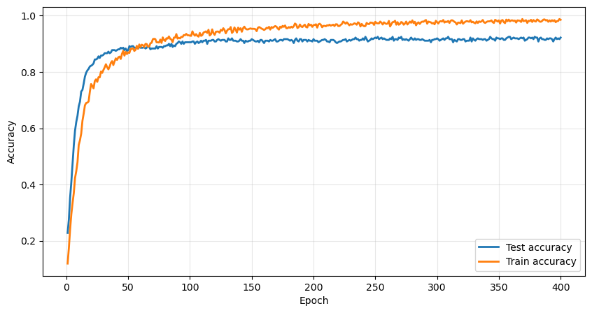
        return x

The data is split 80%/20% into a train and a test set. The training goes well, with the model achieving a final 93% accuracy on the test set. Train/test accuracy training curves

Generating images with backprop

The goal is to generate images that look as much like a digit to the network as possible. This is done by doing something very similar to training, but instead of the network parameters, the input image is modified with gradient descent. In this case, the individual pixels are also clamped between 0 and 16 to match the dataset.

# seed: Array of 64 initial pixels
# target: number between 0-9
# output: Array of 64 modified pixels
def generate_digit(seed, target):
    image = seed.clone() 
    image.requires_grad = True # This is the important part
    image_optimizer = optim.Adam([image], lr=0.1) 
    
    #This is like doing epochs during training
    for step in range(100):
        image_optimizer.zero_grad()
        pred = model(torch.clamp(image, 0, 16)) 
        # Same loss as in training
        loss = F.cross_entropy(pred, torch.tensor(target)) 
        loss.backward()
        image_optimizer.step()
        
    # Clamp s.t. the domain stays the same
    return torch.clamp(image, 0, 16)

With this, we can convert a 0 to be recognized as an 8 by the network

Generateing an 8 from a 0
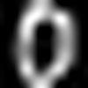
Generating an 8 from zero

But usually, the perception of the network does not align very well with the one of us humans! Here are the optimal digits generated from a black square:

0 1 2 3 4

5 6 7 8 9
Digits created from black squares

If you squint your eyes hard enough you might see some rough shapes for 0, 2, 3, and 5.

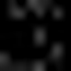
Another thing we can do is generate a bunch of images from noise and average them into a single composite image. In this case for each digit 1000 versions are generated from uniform noise and then averaged:

0 1 2 3 4

5 6 7 8 9
Average digits created from noise

With some more eye squinting, you might even see the 0, 2, 3, 4, 5, 7, and 8!

It is no StableDiffusion, but nonetheless a fun exercise in using backpropagation in an unusual way.

Generating adversarial images

We can also modify the loss function to simultaneously optimize toward a target digit while staying as close to the starting point as possible:

for step in range(100):
    image_optimizer.zero_grad()
    pred = model(torch.clamp(image, 0, 16))

    # This is the same as before
    loss = F.cross_entropy(pred, torch.tensor(target))

    # Additional loss from difference to the original image
    loss += MSE(image, seed) * 2

    loss.backward()
    image_optimizer.step()

For example, the image on the left is correctly read as an 8. But the one on the right, after being altered by the code above, is incorrectly predicted to be a 9.

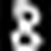
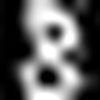
Left: Origianal, read as 8
Right: Adversarial 9 with just a bit of noise

Conclusion

Unfortunately, I was not able to achieve all the initially stated goals because I didn’t achieve 80% accuracy on MNIST with my own backpropagation. I knew this was a pretty ambitious task, but did not expect it to be this hard. Maybe I was a bit spoiled by using well-optimized machine-learning libraries for years now, never appreciating how much slower they could be.
But I’m still happy with the outcome of this project, having learned a lot about backpropagation and gradient descent! Also, the tangent about generating images with backprop was quite fun, mostly because of the visual aspect and not knowing what outcomes to expect.
I think for future learning projects like this it would be a good idea to state the initial goal as something more like “Understand backprop” instead of technical milestones.

The code for this project can be found on GitHub

Cyrill Künzi