Language modeling journey: From bigram prediction and DIY transformers to LLaMA 65B

8 minute read

With all the hype surrounding chatGPT (and now GPT-4), it really bothered me that I don’t have the faintest idea of how language models or transformers work. Fortunately, the Neural Networks: Zero to Hero lecture series that helped me understand backpropagation in my previous post, also covers multiple language modeling techniques. I found that I spend too much time in my last post explaining things that were already covered much better in the lecture. So I’ll try to keep this one shorter.

Goal

The project has the very open-ended goal of “Learning about language models”. I don’t have millions to spend on GPU time to train the next chatGPT, so I’m going to be happy with understanding the underlying theory and training some toy models. These are the rough goals I want to achieve:

Understand how language models are trained
Write my own transformer
Train a GPT language model

Documentation

In this post, I’m going to follow lectures 2 through 7 pretty closely. They start with creating a very simple bigram prediction model and then introduce incrementally more complex models.

Bigram model (729 parameters)

The first step is creating a character-level bigram model: It takes a training text and counts how many times a character follows another. These counts are then normalized and converted to probability distributions. After converting the ASCII characters to integers, all bigrams are counted and the results are stored in a 2D array. In this case, each word is a name and the model will try to predict a new name.

bigram_counts = torch.zeros(27, 27, dtype=torch.int32)

for word in words:
    word = '.' + word + '.'
    for c1, c2 in zip(word, word[1:]):
        bigram_counts[stoi[c1], stoi[c2]] += 1

# Get probability distribution
P_bigram = bigram_counts / bigram_counts.sum(1, keepdims=True)

Something interesting to note is that the words are surrounded by a special character ‘.’ to indicate the start and stop of each sequence. This is useful because generation can be started with a ‘.’ and the model itself can then decide when to stop by generating another ‘.’

After feeding roughly 30’000 names into the model it produces the following probability distribution:

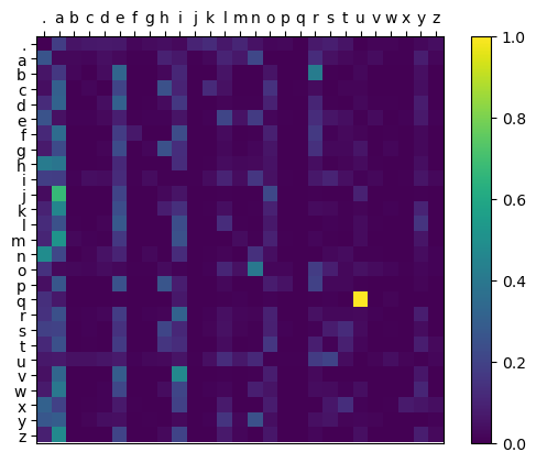
Figure 1: Bigram probability distribution generated by simple counting

As we can see, the model has learned that a lot of names start with ‘a’ and that ‘q’ is almost always followed by ‘u’.

As expected, when we use these probabilities to generate random new names, the results aren’t very good.

.myliena.
.r.
.a.
.ahi.
.grammian.
.n.
.xxonh.
.chaldeiniy.
.bler.
.jaranige.

Because the model only sees the previous character in the sequence, it doesn’t know the length of the generated name. So ‘.a.’ is a perfectly fine choice, as ‘a’ is a common letter at the start and the end of names (see figure 1).

Now with gradient descent (729 parameters)

Instead of explicitly calculating the matrix by counting, the probabilities can be learned with backpropagation and gradient descent. In the following snippet X is the one-hot encoded input character and y is the next character in the sequence. W takes the place of P_bigram from the last section.

W = torch.randn(27, 27, requires_grad=True)

for epoch in range(1000):
    logits = X @ W 
    loss = F.cross_entropy(logits, y)

    W.grad = None
    loss.backward()
    W.data -= 50 * W.grad

After training for a bit, W converges to the following distribution, which looks the same as the one in Figure 1:

Figure 2: Bigram probability distribution generated by backpropagation

This is confirmed when generating random names with the same seed, as the results are exactly the same.

.myliena.
.r.
.a.
.ahi.
.grammian.
.n.
.xxonh.
.chaldeiniy.
.bler.
.jaranige.

Multi-layer perceptron (8’762 parameters)

One straightforward way to improve the model is to increase its context length. In this case, instead of only seeing the previous character, the model is going to see the previous 3 characters. If we just used the previous technique, the resulting 4-dimensional probability matrix would have \(27^4=531'441\) parameters, which is starting to get pretty big. So the purely statistical approach is ditched in favor of a small feed-forward neural network defined like this:

N_EMBEDDINGS = 5
HIDDEN_NEURONS = 200
C = torch.randn((27, N_EMBEDDINGS), requires_grad=True)
W1 = torch.randn((N_EMBEDDINGS * BLOCK_SIZE, HIDDEN_NEURONS), requires_grad=True)
b1 = torch.randn(HIDDEN_NEURONS, requires_grad=True)
W2 = torch.randn((HIDDEN_NEURONS, 27), requires_grad=True)
b2 = torch.randn(27, requires_grad=True)
parameters = [C, W1, b1, W2, b2]

def forward(X):
    embeddings = C[X]
    x = embeddings.view(-1, N_EMBEDDINGS * BLOCK_SIZE)
    x = x @ W1 + b1
    x = torch.tanh(x)
    x = x @ W2 + b2
    return x

This introduces the concept of an embedding which maps each 27-dimensional one-hot encoded input character to a 5-dimensional embedding that is learned together with the rest of the network.
We can take a look at the cosine similarities between all embeddings after training:

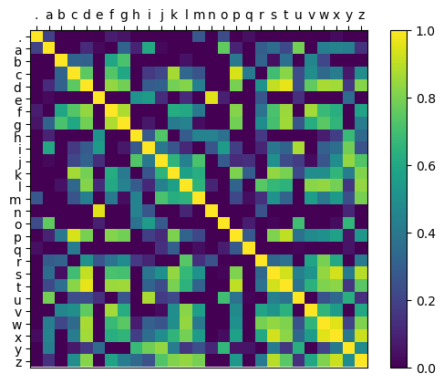
Figure 3: ReLU of the cosine similarities between learned embeddings

It looks like the embeddings of the vowels are often similar to each other and that ‘.’, ‘n’, and ‘q’ have pretty distinct embeddings.

The random names generated with this model are already way better than before:

.mylieke.
.rada.
.erackanolando.
.yusamailem.
.karlymandrah.
.parlif.
.meilae.
.ayy.
.saiora.
.jaylianyyah.

WaveNet (176k parameters)

The next step is extending the context length even further and using another network topology with much more parameters. This topology is a WaveNet introduced in 2016 by Google DeepMind https://arxiv.org/abs/1609.03499. As seen in Figure 4, it uses dilated causal convolutions and was originally created for speech synthesis. In this case, the convolutions are replaced with carefully arranged linear layers and the network is of course used for character prediction.

Figure 4: WaveNet topology source

This particular implementation is very inefficient because the data is occasionally reshaped to create the correct tensor shapes.

class WaveNet(nn.Module):
    def __init__(self, n_embeddings=10, hidden_neurons=200):
        super(WaveNet, self).__init__()
        self.n_embeddings = n_embeddings
        self.hidden_neurons = hidden_neurons
        
        self.embedding = nn.Embedding(27, n_embeddings)
        self.fc1 = nn.Linear(n_embeddings * 2, hidden_neurons)
        self.bn1 = nn.BatchNorm1d(hidden_neurons)
        
        self.fc2 = nn.Linear(hidden_neurons * 2, hidden_neurons)
        self.bn2 = nn.BatchNorm1d(hidden_neurons)
        
        self.fc3 = nn.Linear(hidden_neurons * 2, hidden_neurons)
        self.bn3 = nn.BatchNorm1d(hidden_neurons)
        
        self.fc4 = nn.Linear(hidden_neurons, 27)
        
    def forward(self, x):
        x = self.embedding(x)
        
        x = x.view(-1, 4, self.n_embeddings * 2)
        self.tmp = x
        x = self.fc1(x)
        x = x.swapaxes(1,2)
        x = self.bn1(x)
        x = x.swapaxes(1,2)
        x = torch.tanh(x)
        
        x = x.reshape(-1, 2, self.hidden_neurons * 2)
        x = self.fc2(x)
        x = x.swapaxes(1,2)
        x = self.bn2(x)
        x = x.swapaxes(1,2)
        x = torch.tanh(x)
        
        x = x.reshape(-1, self.hidden_neurons * 2)
        x = self.fc3(x)
        x = self.bn3(x)
        x = torch.tanh(x)
        
        x = self.fc4(x)
       
        return x
    
model = WaveNet(n_embeddings = 20, hidden_neurons=200)

After training this network for a couple of epochs with a decreasing learning rate, the generated names start to sound pretty name-like:

.kynnale.
.obagann.
.evanne.
.jatetton.
.adiliah.
.kiyaen.
.nalar.
.khfi.
.keilei.
.awyana.

Looking at the embedding similarities again, it seems like they are more unique than before. This makes sense considering the dimensionality of the embedding vector has gone up from 5 to 20 Dimensions.

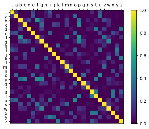
Figure 5: ReLU of the cosine similarities between learned WaveNet embeddings

GPT from scratch (10.7M parameters)

Learning how transformers work was definitely the most exciting part of this project for me! Explaining transformers is no easy task, so I’m not even going to try. If you are interested, I highly recommend watching the lecture.

But I want to quickly show what lies in the heart of a transformer: The self-attention mechanism:
For each input, it generates a query, key, and value that get combined, such that they can exchange information with each other in a very elegant way.

class Head(nn.Module):
    def __init__(self, head_size):
        super().__init__()
        self.key = nn.Linear(n_embeddings, head_size, bias=False)
        self.query = nn.Linear(n_embeddings, head_size, bias=False)
        self.value = nn.Linear(n_embeddings, head_size, bias=False)
        self.register_buffer('tril', torch.tril(torch.ones(block_size, block_size)))
        
        self.dropout = nn.Dropout(dropout)
        
    def forward(self, x):
        B, T, C = x.shape
        k = self.key(x)
        q = self.query(x)
        v = self.value(x)
        
        wei = q @ k.transpose(-2, -1) * k.shape[-1]**-0.5
        wei = wei.masked_fill(self.tril[:T, :T] == 0, float('-inf'))
        wei = F.softmax(wei, dim=-1)
        wei = self.dropout(wei)
        
        x = wei @ v
        
        return x

The final model has 384 embeddings, a context size of 256 characters, and consists of 6 transformer blocks with 6 self-attention heads each. After being trained on the works of Shakespeare for a couple of thousand epochs (on the GPU this time), it produces text like this:

And come to Coriolanus.

CORIOLANUS: I will be so, show; I hope this service As it gives me a word which to practise my lave, When I had rather cry ‘‘twas but a bulk.

MENENIUS: Let’s not pray you.

AUTOLYCUS: I know ‘tis not without the shepherd, not a monster, man.

CORIOLANUS: The poor, Pampey, sir.

CORIOLANUS: Nor thou hast, my lord; there I know the taple I was violently?

CORIOLANUS: Why, that that he were recounted nose, A heart of your lord’st traded, whose eservice we remain With this chance to you did The deputy of such pure complices them Redeem with our love they call and new good to-night.

BRUTUS: I dare now in the voices: here are Acrown the state news.

SICINIUS: You have been in crutching of them, cry on their this?

MENENIUS: Proclam, sir, I shall.

Playing with LLaMA (65B parameters)

While doing this project the weights of Facebooks LLaMa model leaked online in a hilarious way. When looking at their publicly available model, most things seem very similar to the DIY version.

Language models might start having their StableDiffusion moment right now. Seemingly every day there is a new innovation like reducing the model size with quantization or finetuning it to act more like OpenAIs Davinci model. After increasing my WSLs RAM budget to 50GB, downloading the LLaMA weights and quantizing them to 4-bit, I was able to use llama.cpp to run the 65B model on a CPU.
Like with diffusion models, it seems futile to go into much detail here, as the whole landscape will probably look completely different in only a couple of weeks.

Conclusion

Going from having absolutely no clue about LLMs and transformers to understanding the current cutting-edge research was definitely a fun project. Major props have to go to Andrej Karpathy for his amazing lectures that perfectly guided me through this process. I will probably return to this topic soon when the available models and tooling have advanced enough to do DIY fine-tuning.
All code can be found on my GitHub

Cyrill Künzi